Mainnavigation
Subnavigation
BORDER
Pagecontent
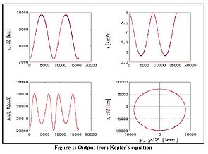
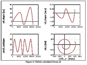
Orbits with Kepler's Equation and Gravity Term J2
The two sets of plots below compare calculated with Kepler's equation with orbits calculated with gravity term J2.
% demoOrbit
% This demo compares the orbits due to Kepler's equations
% that assume that the earth is a point mass, and
% the orbit of a satellite including the effect of the
% gravity term J2 (flattening of Earth at the poles)
%
% Initial condition
% vx vy vz x y z
X0 = [ 0 -8 0 0 0 7200]';

T = 0:10:16000;
lsode_options('absolute',1e-10);
lsode_options('relative',1e-10);
Y0 = lsode('satKepler', X0, T, 0);
R0 = Y0(:,4:6)';
V0 = Y0(:,1:3)';
h  = cross(R0,V0);

Adot = 1/2*sqrt(h(1,:).*h(1,:) + h(2,:).*h(2,:) + h(3,:).*h(3,:));
YJ2  = lsode('satJ2', X0, T, 0);
RJ2  = YJ2(:,4:6)';
VJ2  = YJ2(:,1:3)';
h    = cross(RJ2,VJ2);

AdotJ2 = 1/2*sqrt(h(1,:).*h(1,:) + h(2,:).*h(2,:) + h(3,:).*h(3,:));
x    = Y0(:,4);
y    = Y0(:,5);
z    = Y0(:,6);
vx   = Y0(:,1);
vy   = Y0(:,2);
vz   = Y0(:,3);
r    = sqrt(x.*x + y.*y + z.*z);
v    = sqrt(vx.*vx + vy.*vy + vz.*vz);
xJ2  = YJ2(:,4);
yJ2  = YJ2(:,5);
zJ2  = YJ2(:,6);
vxJ2 = YJ2(:,1);
vyJ2 = YJ2(:,2);
vzJ2 = YJ2(:,3);
rJ2  = sqrt(xJ2.*xJ2 + yJ2.*yJ2 + zJ2.*zJ2);
vJ2  = sqrt(vxJ2.*vxJ2 + vyJ2.*vyJ2 + vzJ2.*vzJ2);
erase

figure(1)
window('221')
plot(T,r,'blue',T,rJ2,'red');
ylabel('r, rJ2 [km]')

window('222')
plot(T,v,'blue',T,vJ2,'red');
ylabel('v [km/s]')
window('223')
plot(T,Adot,'blue',T,AdotJ2,'red')
ylabel('Adot, AdotJ2')

window('224')
plot(y,z,'blue',yJ2,zJ2,'red','grid');
ylabel('z, zJ2 [km]')
xlabel('y, yJ2 [km]')

figure(2)
window('221')
plot(T,rJ2-r,'red');
ylabel('rJ2-rKepler [km]')

window('222')
plot(T,vJ2-v,'red');
ylabel('vJ2-vKepler [km/s]')

window('223')
plot(T,AdotJ2-Adot,'red')
ylabel('AdotJ2-AdotKepler')

window('224')
plot(yJ2-y,zJ2-z,'red','grid');
ylabel('zJ2-z [km]')
xlabel('yJ2-y [km]')